Finding the stellar magnitude limit in an image is not necessarily as straightforward as it, at first, appears. I needed to come up with some non-hand-wavy numbers and thought, ‘No problem, this is easy.’ It turns out that I was wrong. At least for my imagery and what I wanted to say about it.
The ‘proper’ way to calculate the limiting magnitude, it turns out, is to inject synthetic stars of different magnitudes into your imagery and then try to extract them. The magnitude cutoff at which you’re only able to detect 1/2 of the stars at that magnitude is your limiting magnitude. Easy with IRAF (he says with a grin). After struggling mentally with it for a bit, I realized that it wasn’t going to be easy (nor peasy, nor lemon squeezy) at all, so I’d look for another way.
The images that I wanted to work with were from the EMCCD cameras that are collecting the data for my PhD project. They’re of a moderate field-of-view (ca. 15°x15°) and tend to have lots of stars. In a quick visual scan, one can pick out stars (sometimes) down to 12th magnitude. Not bad for a 50 mm photographic lens running at 32 fps. But is that the limiting magnitude? As it turns out, nope.
The wavelength response of the unfiltered EMCCD system is fairly wide. It goes from about 375 nm out to around a μm (the lens is not responsive beyond about 950 nm), so tying it to a particular filter is challenging. Which means that we can’t really compare our measured magnitudes directly to, say, the V magnitudes that might be given in our comparison catalog. Ideally, we’d look for a comparison catalog that gives magnitudes in a similar passband as our system. It turns out that the Gaia G passband is a reasonably close match.
The procedure
- Correct your image for bias, dark, and flat
- Find the plate solution for your image (try Astrometry.net or SCAMP)
- Run SExtractor on the image to create a catalog of sources
- Run some python code to cross-check the detected objects against Gaia DR2
- Look at the plot of instrumental vs Gaia magnitudes and decide where real object detections falls off and call that your ‘limit’
The code will provide a handy plot showing instrumental magnitude vs Gaia G-band magnitude. What you’ll see is a trend that drops off at some magnitude. The point at which it drops off is the ultimate limiting magnitude.
Setting up SCAMP and SExtractor
More to come…
Downloading Gaia
When I first did this exercise I queried (using astroquery) the Gaia DR2 online database for each detected source separately. With a couple of thousand sources in each image, this can take a lot of time. A better solution is to download a larger area of the catalog and then query that directly. There are a number of different places to do this, but the one that I used can be found here…
http://jvo.nao.ac.jp/portal/gaia/dr2.do
As the first step of the process you select the fields that you want to retrieve. I chose: source_id, ra, dec, parallax (no sure why I bothered), phot_g_mean_mag, phot_bp_mean_mag, and phot_rp_mean_mag. Next, I chose a field radius of 45 degrees centered on an RA/Dec of 0/90 and proceeded with the download.
import matplotlib.pyplot as plt
import sys
import pandas as pd

filename = 'test.cat'
# filename = sys.argv[1]
gfilename = "./GaiaDR2_45to90-M13.psv"

SR = 0.03 # Search distance in degrees

data = pd.read_csv(filename, delim_whitespace=True, skiprows=14)
data.columns = ['Number','XWIN','YWIN','XWORLD','YWORLD','MAG','MAGERROR','FLUX','FLUXERROR','FLUXRADIUS','FWHM','BACKGROUND','RA','DEC']

gdata = pd.read_csv(gfilename, delimiter="|", skiprows=4, low_memory=False)
gdata.columns = ["ID","gRA","gDEC","PAR","gMAG","bMAG","rMAG"] # Make sure that these columns are the ones downloaded from the data server

gdata = gdata.drop('ID', axis=1) # May as well get rid of the ID column

data['BMAG'] = 99
data['GMAG'] = 99
data['RMAG'] = 99

for i in range(len(data.index)):
    RA = data.loc[i,'RA']
    DEC = data.loc[i,'DEC']

    df = gdata[(gdata.gRA < (RA+SR))]
    df = df[(df.gRA > (RA-SR))]
    df = df[(df.gDEC < (DEC+SR))]
    df = df[(df.gDEC > (DEC-SR))]
    df.sort_values(by=["gMAG"], ascending=True, inplace=True)
    df.reset_index(drop=True, inplace=True)

    if len(df.index)>1:
        data.loc[i,'BMAG'] = df.loc[0]['bMAG']
        data.loc[i,'GMAG'] = df.loc[0]['gMAG']
        data.loc[i,'RMAG'] = df.loc[0]['rMAG']

print('Pickling...')
data.to_pickle('out.pkl')
print('Pickled...')

print('Plotting figure...')

plt.figure(figsize=(14,10))

plt.scatter(data['GMAG'],data['MAG'], color='green')

plt.xlabel('Gaia DR2 G-band Magnitude', size=15)
plt.ylabel('Instrumental Magnitude', size=15)
plt.xlim(4,13)
plt.ylim(-15,-2)
plt.tight_layout()
plt.savefig('Imag-vs-Gmag.png', dpi=300)

plt.show()
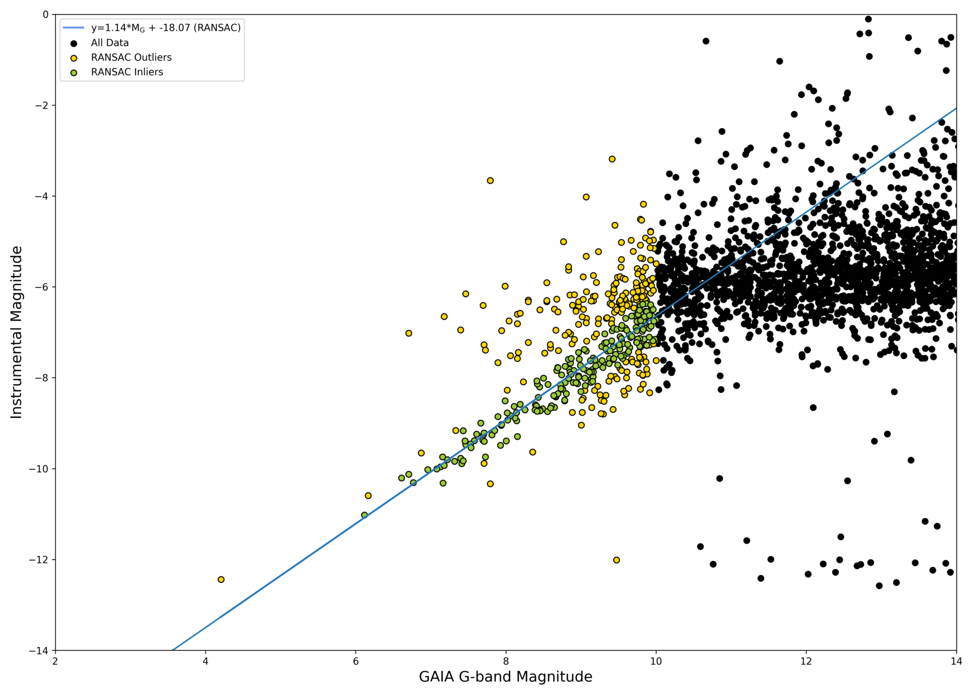
The above code will save the results in a .pkl file and produce a rudimentary plot showing the SExtractor instrumental magnitude plotted against the Gaia g-band magnitude. Since you’ve got the pickle file, you can always play with it a bit and make a more informative plot like the one below. The example data given below is from an image from my finder scope project using a 50 mm f1.4 lens while running at 25 fps. In order to calculate a quick and dirty instrumental-to-g transformation, I’ve taken stars with a g-band magnitude less than 10 and fit a line through them using a RANSAC regressor. What’s immediately apparent from the plot is that there is a pretty convincing trend through the data. Two actually. The first slopes upwards until a break is reached at about 10.8 Gaia g-band magnitude. After this point, the trend is flat. So, I’ll take the limiting magnitude as 10.8 for this setup. As this is an unfiltered system being compared to a known passband, there is a a fair bit of scatter and I’m not sure that we could do much better with the more precise synthetic injection method.
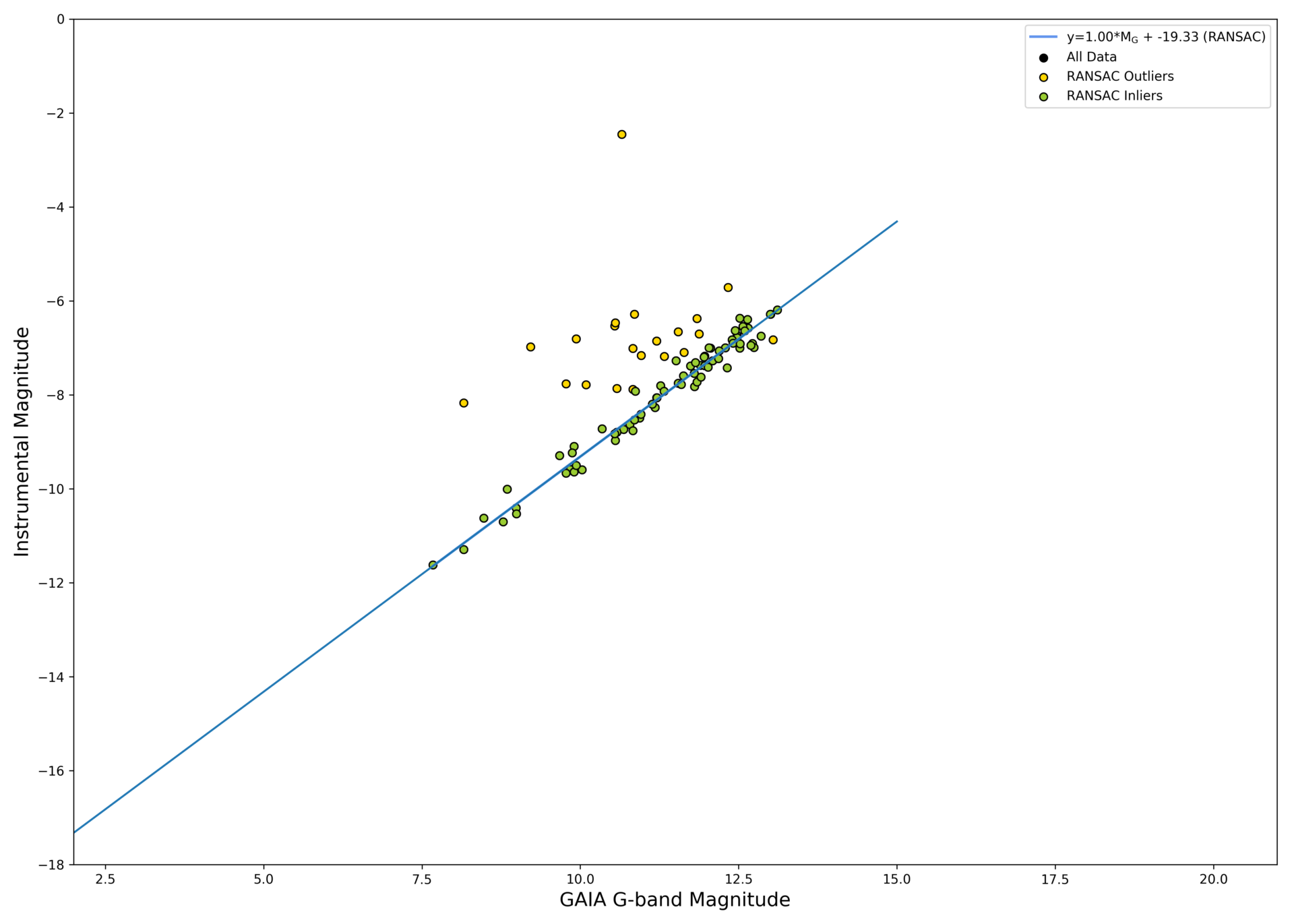
Two additional examples use data from a 50 cm f3 telescope equipped with an FLI Kepler 4040. The first is a 25 ms exposure while the second is a longer 10 s exposure. Although with the short exposure there are relatively few detections (less than 100 in total), there are still enough to define a trend through the data. In this case, the limiting magnitude is about M13. There is no flattening of the curve and there are no detections fainter than this limit.
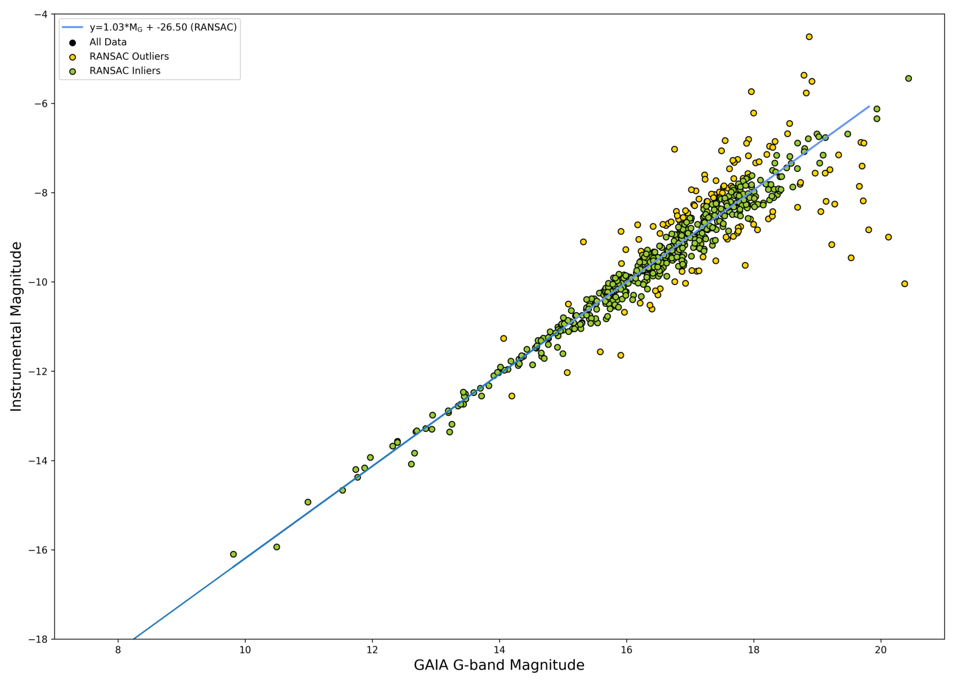
With a longer exposure, there are naturally more detections and the trend is better-defined. In the figure below we see that there is actually a deviation from the dominant trend for detections below about M18.5. Yes, there are likely a couple of real detections that are fainter (down to M20) but there are also quite a few missed objects between M18.5 and M20.
Improvements can be made by simply counting the number of number of objects that should be made for a given magnitude within the field-of-view and comparing it to those that are actually found by SExtractor.
Summary
More to come…